You can run this notebook in a live session ![]() or view it on Github.
or view it on Github.
Table of Contents
1 Compare weighted and unweighted mean temperature
1.0.1 Data
1.0.2 Creating weights
1.0.3 Weighted mean
1.0.4 Plot: comparison with unweighted mean
Compare weighted and unweighted mean temperature#
Author: Mathias Hauser
We use the air_temperature example dataset to calculate the area-weighted temperature over its domain. This dataset has a regular latitude/ longitude grid, thus the grid cell area decreases towards the pole. For this grid we can use the cosine of the latitude as proxy for the grid cell area.
[1]:
%matplotlib inline

import cartopy.crs as ccrs
import matplotlib.pyplot as plt
import numpy as np

import xarray as xr
Data#
Load the data, convert to celsius, and resample to daily values
[2]:
ds = xr.tutorial.load_dataset("air_temperature")

# to celsius
air = ds.air - 273.15

# resample from 6-hourly to daily values
air = air.resample(time="D").mean()

air
[2]:
<xarray.DataArray 'air' (time: 730, lat: 25, lon: 53)> Size: 8MB
array([[[-31.2775, -30.85  , -30.475 , ..., -39.7775, -37.975 ,
         -35.475 ],
        [-28.575 , -28.5775, -28.875 , ..., -41.9025, -40.325 ,
         -36.85  ],
        [-19.15  , -19.9275, -21.3275, ..., -41.675 , -39.455 ,
         -34.525 ],
        ...,
        [ 23.15  ,  22.825 ,  22.85  , ...,  22.7475,  22.17  ,
          21.795 ],
        [ 23.175 ,  23.575 ,  23.5925, ...,  23.0225,  22.85  ,
          22.3975],
        [ 23.47  ,  23.845 ,  23.95  , ...,  23.8725,  23.8975,
          23.8225]],

       [[-29.55  , -29.65  , -29.85  , ..., -34.1775, -32.3525,
         -30.0775],
        [-25.3275, -25.95  , -26.9275, ..., -37.225 , -36.5525,
         -34.55  ],
        [-19.6275, -21.0775, -22.8525, ..., -35.4525, -34.2775,
         -31.25  ],
...
        [ 23.215 ,  22.265 ,  22.015 , ...,  23.74  ,  23.195 ,
          22.195 ],
        [ 24.3675,  24.515 ,  23.895 , ...,  23.415 ,  22.995 ,
          22.27  ],
        [ 25.4175,  25.5925,  25.1925, ...,  23.6425,  23.19  ,
          22.72  ]],

       [[-28.935 , -29.535 , -30.385 , ..., -29.41  , -28.96  ,
         -28.46  ],
        [-23.835 , -24.06  , -24.56  , ..., -32.585 , -31.635 ,
         -30.035 ],
        [-10.21  , -10.785 , -11.435 , ..., -33.685 , -31.035 ,
         -27.135 ],
        ...,
        [ 21.69  ,  21.99  ,  23.49  , ...,  22.265 ,  22.015 ,
          21.415 ],
        [ 23.39  ,  24.44  ,  24.94  , ...,  22.415 ,  22.315 ,
          21.64  ],
        [ 24.84  ,  25.59  ,  25.54  , ...,  23.065 ,  22.715 ,
          22.39  ]]], shape=(730, 25, 53))
Coordinates:
  * lat      (lat) float32 100B 75.0 72.5 70.0 67.5 65.0 ... 22.5 20.0 17.5 15.0
  * lon      (lon) float32 212B 200.0 202.5 205.0 207.5 ... 325.0 327.5 330.0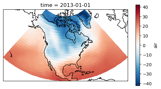
* time (time) datetime64[ns] 6kB 2013-01-01 2013-01-02 ... 2014-12-31Plot the first timestep:
[3]:
projection = ccrs.LambertConformal(central_longitude=-95, central_latitude=45)

f, ax = plt.subplots(subplot_kw=dict(projection=projection))

air.isel(time=0).plot(transform=ccrs.PlateCarree(), cbar_kwargs=dict(shrink=0.7))
ax.coastlines()
[3]:
<cartopy.mpl.feature_artist.FeatureArtist at 0x7f86fb5330e0>
/home/docs/checkouts/readthedocs.org/user_builds/xray/conda/10526/lib/python3.13/site-packages/cartopy/io/__init__.py:241: DownloadWarning: Downloading: https://naturalearth.s3.amazonaws.com/110m_physical/ne_110m_coastline.zip
  warnings.warn(f'Downloading: {url}', DownloadWarning)
Creating weights#
For a rectangular grid the cosine of the latitude is proportional to the grid cell area.
[4]:
weights = np.cos(np.deg2rad(air.lat))
weights.name = "weights"
weights
[4]:
<xarray.DataArray 'weights' (lat: 25)> Size: 100B
array([0.25881907, 0.30070582, 0.34202015, 0.38268346, 0.42261827,
       0.4617486 , 0.49999997, 0.5372996 , 0.57357645, 0.6087614 ,
       0.6427876 , 0.67559016, 0.70710677, 0.7372773 , 0.76604444,
       0.7933533 , 0.81915206, 0.8433914 , 0.8660254 , 0.8870108 ,
       0.90630776, 0.9238795 , 0.9396926 , 0.95371693, 0.9659258 ],
      dtype=float32)
Coordinates:
  * lat      (lat) float32 100B 75.0 72.5 70.0 67.5 65.0 ... 22.5 20.0 17.5 15.0
Attributes:
    standard_name:  latitude
    long_name:      Latitude
    units:          degrees_north
axis: YWeighted mean#
[5]:
air_weighted = air.weighted(weights)
air_weighted
[5]:
DataArrayWeighted with weights along dimensions: lat
[6]:
weighted_mean = air_weighted.mean(("lon", "lat"))
weighted_mean
[6]:
<xarray.DataArray 'air' (time: 730)> Size: 6kB
array([ 6.09239733,  5.52798843,  5.65128653,  5.78623494,  5.91176272,
        5.68343433,  5.97670966,  6.45671969,  6.57106097,  6.50464312,
        6.13489632,  5.92686336,  5.82681984,  5.72286499,  5.5780027 ,
        5.4655198 ,  5.09123756,  4.98601216,  5.22862495,  5.25165848,
        5.42772269,  5.38779008,  5.43389566,  5.36439691,  5.46853466,
        5.22902604,  5.35028182,  5.34182714,  5.37266728,  5.35951009,
        5.14033313,  5.05556218,  5.07246082,  5.23521611,  5.31848177,
        5.49917179,  5.72088266,  5.72860999,  5.76080587,  5.82555821,
        6.26850058,  6.43689923,  6.51022854,  6.56476304,  6.60878065,
        6.4212634 ,  5.91473879,  5.55467421,  5.32921328,  5.33590339,
        5.07058623,  5.28373323,  5.59521539,  6.0546562 ,  6.53072732,
        6.50741412,  6.3917386 ,  6.39512352,  6.39808504,  6.5293698 ,
        6.47710739,  6.53576171,  6.69251592,  6.67736523,  6.5116295 ,
        6.44702956,  6.86037431,  7.43753239,  7.69810276,  7.48425856,
        7.25818587,  7.13595535,  7.0934042 ,  7.26708315,  7.3485328 ,
        7.3217832 ,  7.2211416 ,  7.21292338,  7.28403842,  7.54337582,
        7.85436875,  8.11583664,  8.26189315,  8.11161849,  8.21912214,
        8.35870973,  8.71614382,  9.15188087,  9.37003955,  9.41586084,
        9.07343345,  8.82065128,  8.8046395 ,  8.85637743,  9.06744766,
        9.40714644,  9.69692473,  9.7420737 ,  9.65961453,  9.69560854,
...
       17.48427167, 17.33174925, 17.20261324, 17.06820928, 16.91004629,
       16.53691939, 16.13330631, 16.05550705, 16.10007907, 15.90940242,
       15.76408748, 15.63148333, 15.82774318, 16.0262186 , 16.31986814,
       16.15644458, 15.89844257, 15.83085789, 15.81007381, 15.58978913,
       15.30961597, 15.10517123, 14.96467422, 14.96696909, 14.90459818,
       14.61065649, 14.33011118, 14.25560953, 14.31402823, 13.94010009,
       13.75886281, 13.82086244, 14.02183067, 13.88818562, 13.72470701,
       13.19087298, 12.99514545, 12.66983911, 12.58503039, 12.37766749,
       12.17865015, 12.08231079, 11.87420288, 11.66016425, 11.60113381,
       11.55860859, 11.18384495, 11.23734384, 11.09191512, 10.47219025,
        9.89890944,  9.43123626,  9.49159156,  9.6886162 ,  9.99857146,
        9.79354814,  9.31528239,  9.25993118,  9.38499228,  9.343001  ,
        9.20258339,  9.47232595,  9.42420929,  9.05067273,  8.56818269,
        7.71914511,  7.33122037,  7.45129757,  7.42358734,  7.51879348,
        7.4950339 ,  7.62386211,  8.08324312,  8.04912883,  8.02726716,
        8.06961004,  7.91252824,  8.04294281,  8.34480776,  8.50706783,
        8.70819522,  8.60494761,  8.31246173,  8.2572366 ,  7.98413779,
        7.69330548,  7.42197294,  7.43523459,  7.48295603,  7.64284165,
        7.90846595,  8.03612978,  7.62541613,  7.75331309,  7.85042281,
        7.62129868,  6.84733814,  6.45026245,  5.98523748,  5.58057559])
Coordinates: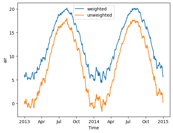
* time (time) datetime64[ns] 6kB 2013-01-01 2013-01-02 ... 2014-12-31Plot: comparison with unweighted mean#
Note how the weighted mean temperature is higher than the unweighted.
[7]:
weighted_mean.plot(label="weighted")
air.mean(("lon", "lat")).plot(label="unweighted")

plt.legend()
[7]:
<matplotlib.legend.Legend at 0x7f86fb5ce270>