Other File Formats

This page covers additional file formats and data sources supported by xarray beyond netCDF/HDF5 and Zarr.

Kerchunk

Kerchunk is a Python library that allows you to access chunked and compressed data formats (such as NetCDF3, NetCDF4, HDF5, GRIB2, TIFF & FITS), many of which are primary data formats for many data archives, by viewing the whole archive as an ephemeral Zarr dataset which allows for parallel, chunk-specific access.

Instead of creating a new copy of the dataset in the Zarr spec/format or downloading the files locally, Kerchunk reads through the data archive and extracts the byte range and compression information of each chunk and saves as a reference. These references are then saved as json files or parquet (more efficient) for later use. You can view some of these stored in the references directory here.

Note

These references follow this specification. Packages like kerchunk and virtualizarr help in creating and reading these references.

Reading these data archives becomes really easy with kerchunk in combination with xarray, especially when these archives are large in size. A single combined reference can refer to thousands of the original data files present in these archives. You can view the whole dataset with from this combined reference using the above packages.

The following example shows opening a single json reference to the saved_on_disk.h5 file created above. If the file were instead stored remotely (e.g. s3://saved_on_disk.h5) you can use storage_options that are used to configure fsspec:

ds_kerchunked = xr.open_dataset(
    "./combined.json",
    engine="kerchunk",
    storage_options={},
)

ds_kerchunked

<xarray.Dataset> Size: 232B
Dimensions:  (x: 4, y: 5)
Coordinates:
  * x        (x) int64 32B 10 20 30 40
  * y        (y) datetime64[ns] 40B 2000-01-01 2000-01-02 ... 2000-01-05
Data variables:
    foo      (x, y) float64 160B ...

xarray.Dataset

• Dimensions:
  • x: 4
  • y: 5
• Coordinates: (2)
  • x
    (x)
    int64
    10 20 30 40

    array([10, 20, 30, 40])

  • y
    (y)
    datetime64[ns]
    2000-01-01 ... 2000-01-05

    array(['2000-01-01T00:00:00.000000000', '2000-01-02T00:00:00.000000000',
           '2000-01-03T00:00:00.000000000', '2000-01-04T00:00:00.000000000',
           '2000-01-05T00:00:00.000000000'], dtype='datetime64[ns]')

• Data variables: (1)
  • foo
    (x, y)
    float64
    ...

    [20 values with dtype=float64]

• Indexes: (2)
  • x
    PandasIndex

    PandasIndex(Index([10, 20, 30, 40], dtype='int64', name='x'))

  • y
    PandasIndex

    PandasIndex(DatetimeIndex(['2000-01-01', '2000-01-02', '2000-01-03', '2000-01-04',
                   '2000-01-05'],
                  dtype='datetime64[ns]', name='y', freq=None))

• Attributes: (0)

Note

You can refer to the project pythia kerchunk cookbook and the pangeo guide on kerchunk for more information.

Iris

The Iris tool allows easy reading of common meteorological and climate model formats (including GRIB and UK MetOffice PP files) into Cube objects which are in many ways very similar to DataArray objects, while enforcing a CF-compliant data model.

DataArray to_iris and from_iris

If iris is installed, xarray can convert a DataArray into a Cube using DataArray.to_iris():

da = xr.DataArray(
    np.random.rand(4, 5),
    dims=["x", "y"],
    coords=dict(x=[10, 20, 30, 40], y=pd.date_range("2000-01-01", periods=5)),
)

cube = da.to_iris()
print(cube)

unknown / (unknown)                 (x: 4; y: 5)
    Dimension coordinates:
        x                             x     -
        y                             -     x

Conversely, we can create a new DataArray object from a Cube using DataArray.from_iris():

da_cube = xr.DataArray.from_iris(cube)
da_cube

<xarray.DataArray (x: 4, y: 5)> Size: 160B
array([[0.12696983, 0.96671784, 0.26047601, 0.89723652, 0.37674972],
       [0.33622174, 0.45137647, 0.84025508, 0.12310214, 0.5430262 ],
       [0.37301223, 0.44799682, 0.12944068, 0.85987871, 0.82038836],
       [0.35205354, 0.2288873 , 0.77678375, 0.59478359, 0.13755356]])
Coordinates:
  * x        (x) int64 32B 10 20 30 40
  * y        (y) datetime64[ns] 40B 2000-01-01 2000-01-02 ... 2000-01-05

xarray.DataArray

• x: 4
• y: 5

• 0.127 0.9667 0.2605 0.8972 0.3767 ... 0.2289 0.7768 0.5948 0.1376

  array([[0.12696983, 0.96671784, 0.26047601, 0.89723652, 0.37674972],
         [0.33622174, 0.45137647, 0.84025508, 0.12310214, 0.5430262 ],
         [0.37301223, 0.44799682, 0.12944068, 0.85987871, 0.82038836],
         [0.35205354, 0.2288873 , 0.77678375, 0.59478359, 0.13755356]])

• Coordinates: (2)
  • x
    (x)
    int64
    10 20 30 40

    array([10, 20, 30, 40])

  • y
    (y)
    datetime64[ns]
    2000-01-01 ... 2000-01-05

    array(['2000-01-01T00:00:00.000000000', '2000-01-02T00:00:00.000000000',
           '2000-01-03T00:00:00.000000000', '2000-01-04T00:00:00.000000000',
           '2000-01-05T00:00:00.000000000'], dtype='datetime64[ns]')

• Indexes: (2)
  • x
    PandasIndex

    PandasIndex(Index([10, 20, 30, 40], dtype='int64', name='x'))

  • y
    PandasIndex

    PandasIndex(DatetimeIndex(['2000-01-01', '2000-01-02', '2000-01-03', '2000-01-04',
                   '2000-01-05'],
                  dtype='datetime64[ns]', name='y', freq=None))

• Attributes: (0)

Ncdata

Ncdata provides more sophisticated means of transferring data, including entire datasets. It uses the file saving and loading functions in both projects to provide a more “correct” translation between them, but still with very low overhead and not using actual disk files.

Here we load an xarray dataset and convert it to Iris cubes:

ds = xr.tutorial.open_dataset("air_temperature_gradient")
cubes = ncdata.iris_xarray.cubes_from_xarray(ds)
print(cubes)

0: $∂T/∂x$ / (°C/m)                    (time: 2920; latitude: 25; longitude: 53)
1: $∂T/∂y$ / (°C/m)                    (time: 2920; latitude: 25; longitude: 53)
2: 4xDaily Air temperature at sigma level 995 / (degK) (time: 2920; latitude: 25; longitude: 53)

/home/docs/checkouts/readthedocs.org/user_builds/xray/conda/10526/lib/python3.13/site-packages/ncdata/iris_xarray.py:52: SerializationWarning: saving variable Tair with floating point data as an integer dtype without any _FillValue to use for NaNs
  ncdata = from_xarray(xrds, **xr_save_kwargs)

print(cubes[1])

$∂T/∂y$ / (°C/m)                    (time: 2920; latitude: 25; longitude: 53)
    Dimension coordinates:
        time                             x               -              -
        latitude                         -               x              -
        longitude                        -               -              x
    Attributes:
        Conventions                 'COARDS'
        description                 'Data is from NMC initialized reanalysis\n(4x/day).  These are the 0.9950 ...'
        platform                    'Model'
        references                  'http://www.esrl.noaa.gov/psd/data/gridded/data.ncep.reanalysis.html'
        title                       '4x daily NMC reanalysis (1948)'

And we can convert the cubes back to an xarray dataset:

# ensure dataset-level and variable-level attributes loaded correctly
iris.FUTURE.save_split_attrs = True

ds = ncdata.iris_xarray.cubes_to_xarray(cubes)
ds

<xarray.Dataset> Size: 62MB
Dimensions:  (time: 2920, lat: 25, lon: 53)
Coordinates:
    time     (time) datetime64[ns] 23kB dask.array<chunksize=(2920,), meta=np.ndarray>
    lat      (lat) float32 100B dask.array<chunksize=(25,), meta=np.ndarray>
    lon      (lon) float32 212B dask.array<chunksize=(53,), meta=np.ndarray>
Data variables:
    dTdx     (time, lat, lon) float32 15MB dask.array<chunksize=(2920, 25, 53), meta=numpy.ma.MaskedArray>
    dTdy     (time, lat, lon) float32 15MB dask.array<chunksize=(2920, 25, 53), meta=numpy.ma.MaskedArray>
    Tair     (time, lat, lon) float64 31MB dask.array<chunksize=(2920, 25, 53), meta=numpy.ma.MaskedArray>
Attributes:
    Conventions:  CF-1.7
    description:  Data is from NMC initialized reanalysis\n(4x/day).  These a...
    platform:     Model
    references:   http://www.esrl.noaa.gov/psd/data/gridded/data.ncep.reanaly...
    title:        4x daily NMC reanalysis (1948)

xarray.Dataset

• Dimensions:
  • time: 2920
  • lat: 25
  • lon: 53
• Coordinates: (3)
  • time
    (time)
    datetime64[ns]
    dask.array<chunksize=(2920,), meta=np.ndarray>

    axis :

    T

    standard_name :

    time

    long_name :

    Time

    Array Chunk Bytes 22.81 kiB 22.81 kiB Shape (2920,) (2920,) Dask graph 1 chunks in 3 graph layers Data type datetime64[ns] numpy.ndarray

  • lat
    (lat)
    float32
    dask.array<chunksize=(25,), meta=np.ndarray>

    axis :

    Y

    units :

    degrees_north

    standard_name :

    latitude

    long_name :

    Latitude

    Array Chunk Bytes 100 B 100 B Shape (25,) (25,) Dask graph 1 chunks in 2 graph layers Data type float32 numpy.ndarray

  • lon
    (lon)
    float32
    dask.array<chunksize=(53,), meta=np.ndarray>

    axis :

    X

    units :

    degrees_east

    standard_name :

    longitude

    long_name :

    Longitude

    Array Chunk Bytes 212 B 212 B Shape (53,) (53,) Dask graph 1 chunks in 2 graph layers Data type float32 numpy.ndarray

• Data variables: (3)
  • dTdx
    (time, lat, lon)
    float32
    dask.array<chunksize=(2920, 25, 53), meta=numpy.ma.MaskedArray>

    long_name :

    $∂T/∂x$

    units :

    °C/m

    Array Chunk Bytes 14.76 MiB 14.76 MiB Shape (2920, 25, 53) (2920, 25, 53) Dask graph 1 chunks in 6 graph layers Data type float32 numpy.ma.MaskedArray

  • dTdy
    (time, lat, lon)
    float32
    dask.array<chunksize=(2920, 25, 53), meta=numpy.ma.MaskedArray>

    long_name :

    $∂T/∂y$

    units :

    °C/m

    Array Chunk Bytes 14.76 MiB 14.76 MiB Shape (2920, 25, 53) (2920, 25, 53) Dask graph 1 chunks in 6 graph layers Data type float32 numpy.ma.MaskedArray

  • Tair
    (time, lat, lon)
    float64
    dask.array<chunksize=(2920, 25, 53), meta=numpy.ma.MaskedArray>

    long_name :

    4xDaily Air temperature at sigma level 995

    units :

    degK

    GRIB_id :

    11

    GRIB_name :

    TMP

    actual_range :

    [185.16 322.1 ]

    dataset :

    NMC Reanalysis

    level_desc :

    Surface

    parent_stat :

    Other

    precision :

    2

    statistic :

    Individual Obs

    var_desc :

    Air temperature

    Array Chunk Bytes 29.52 MiB 29.52 MiB Shape (2920, 25, 53) (2920, 25, 53) Dask graph 1 chunks in 14 graph layers Data type float64 numpy.ma.MaskedArray

• Indexes: (0)
• Attributes: (5)

  Conventions :

  CF-1.7

  description :

  Data is from NMC initialized reanalysis (4x/day). These are the 0.9950 sigma level values.

  platform :

  Model

  references :

  http://www.esrl.noaa.gov/psd/data/gridded/data.ncep.reanalysis.html

  title :

  4x daily NMC reanalysis (1948)

Ncdata can also adjust file data within load and save operations, to fix data loading problems or provide exact save formatting without needing to modify files on disk. See for example : ncdata usage examples

OPeNDAP

Xarray includes support for OPeNDAP (via the netCDF4 library or Pydap), which lets us access large datasets over HTTP.

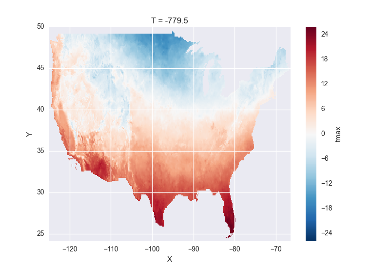
For example, we can open a connection to GBs of weather data produced by the PRISM project, and hosted by IRI at Columbia:

remote_data = xr.open_dataset(
    "http://iridl.ldeo.columbia.edu/SOURCES/.OSU/.PRISM/.monthly/dods",
    decode_times=False,
    )
remote_data

<xarray.Dataset>
Dimensions:  (T: 1422, X: 1405, Y: 621)
Coordinates:
  * X        (X) float32 -125.0 -124.958 -124.917 -124.875 -124.833 -124.792 -124.75 ...
  * T        (T) float32 -779.5 -778.5 -777.5 -776.5 -775.5 -774.5 -773.5 -772.5 -771.5 ...
  * Y        (Y) float32 49.9167 49.875 49.8333 49.7917 49.75 49.7083 49.6667 49.625 ...
Data variables:
    ppt      (T, Y, X) float64 ...
    tdmean   (T, Y, X) float64 ...
    tmax     (T, Y, X) float64 ...
    tmin     (T, Y, X) float64 ...
Attributes:
    Conventions: IRIDL
    expires: 1375315200

Note

Like many real-world datasets, this dataset does not entirely follow CF conventions. Unexpected formats will usually cause xarray’s automatic decoding to fail. The way to work around this is to either set decode_cf=False in open_dataset to turn off all use of CF conventions, or by only disabling the troublesome parser. In this case, we set decode_times=False because the time axis here provides the calendar attribute in a format that xarray does not expect (the integer 360 instead of a string like '360_day').

We can select and slice this data any number of times, and nothing is loaded over the network until we look at particular values:

tmax = remote_data["tmax"][:500, ::3, ::3]
tmax

<xarray.DataArray 'tmax' (T: 500, Y: 207, X: 469)>
[48541500 values with dtype=float64]
Coordinates:
  * Y        (Y) float32 49.9167 49.7917 49.6667 49.5417 49.4167 49.2917 ...
  * X        (X) float32 -125.0 -124.875 -124.75 -124.625 -124.5 -124.375 ...
  * T        (T) float32 -779.5 -778.5 -777.5 -776.5 -775.5 -774.5 -773.5 ...
Attributes:
    pointwidth: 120
    standard_name: air_temperature
    units: Celsius_scale
    expires: 1443657600

# the data is downloaded automatically when we make the plot
tmax[0].plot()

Some servers require authentication before we can access the data. Pydap uses a Requests session object (which the user can pre-define), and this session object can recover authentication`__ credentials from a locally stored .netrc file. For example, to connect to a server that requires NASA’s URS authentication, with the username/password credentials stored on a locally accessible .netrc, access to OPeNDAP data should be as simple as this:

import xarray as xr
import requests

my_session = requests.Session()

ds_url = 'https://gpm1.gesdisc.eosdis.nasa.gov/opendap/hyrax/example.nc'

ds = xr.open_dataset(ds_url, session=my_session, engine="pydap")

Moreover, a bearer token header can be included in a Requests session object, allowing for token-based authentication which OPeNDAP servers can use to avoid some redirects.

Lastly, OPeNDAP servers may provide endpoint URLs for different OPeNDAP protocols, DAP2 and DAP4. To specify which protocol between the two options to use, you can replace the scheme of the url with the name of the protocol. For example:

# dap2 url
ds_url = 'dap2://gpm1.gesdisc.eosdis.nasa.gov/opendap/hyrax/example.nc'

# dap4 url
ds_url = 'dap4://gpm1.gesdisc.eosdis.nasa.gov/opendap/hyrax/example.nc'

While most OPeNDAP servers implement DAP2, not all servers implement DAP4. It is recommended to check if the URL you are using supports DAP4 by checking the URL on a browser.

Pickle

The simplest way to serialize an xarray object is to use Python’s built-in pickle module:

import pickle

# use the highest protocol (-1) because it is way faster than the default
# text based pickle format
pkl = pickle.dumps(ds, protocol=-1)

pickle.loads(pkl)

<xarray.Dataset> Size: 62MB
Dimensions:  (time: 2920, lat: 25, lon: 53)
Coordinates:
    time     (time) datetime64[ns] 23kB dask.array<chunksize=(2920,), meta=np.ndarray>
    lat      (lat) float32 100B dask.array<chunksize=(25,), meta=np.ndarray>
    lon      (lon) float32 212B dask.array<chunksize=(53,), meta=np.ndarray>
Data variables:
    dTdx     (time, lat, lon) float32 15MB dask.array<chunksize=(2920, 25, 53), meta=numpy.ma.MaskedArray>
    dTdy     (time, lat, lon) float32 15MB dask.array<chunksize=(2920, 25, 53), meta=numpy.ma.MaskedArray>
    Tair     (time, lat, lon) float64 31MB dask.array<chunksize=(2920, 25, 53), meta=numpy.ma.MaskedArray>
Attributes:
    Conventions:  CF-1.7
    description:  Data is from NMC initialized reanalysis\n(4x/day).  These a...
    platform:     Model
    references:   http://www.esrl.noaa.gov/psd/data/gridded/data.ncep.reanaly...
    title:        4x daily NMC reanalysis (1948)

xarray.Dataset

• Dimensions:
  • time: 2920
  • lat: 25
  • lon: 53
• Coordinates: (3)
  • time
    (time)
    datetime64[ns]
    dask.array<chunksize=(2920,), meta=np.ndarray>

    axis :

    T

    standard_name :

    time

    long_name :

    Time

    Array Chunk Bytes 22.81 kiB 22.81 kiB Shape (2920,) (2920,) Dask graph 1 chunks in 3 graph layers Data type datetime64[ns] numpy.ndarray

  • lat
    (lat)
    float32
    dask.array<chunksize=(25,), meta=np.ndarray>

    axis :

    Y

    units :

    degrees_north

    standard_name :

    latitude

    long_name :

    Latitude

    Array Chunk Bytes 100 B 100 B Shape (25,) (25,) Dask graph 1 chunks in 2 graph layers Data type float32 numpy.ndarray

  • lon
    (lon)
    float32
    dask.array<chunksize=(53,), meta=np.ndarray>

    axis :

    X

    units :

    degrees_east

    standard_name :

    longitude

    long_name :

    Longitude

    Array Chunk Bytes 212 B 212 B Shape (53,) (53,) Dask graph 1 chunks in 2 graph layers Data type float32 numpy.ndarray

• Data variables: (3)
  • dTdx
    (time, lat, lon)
    float32
    dask.array<chunksize=(2920, 25, 53), meta=numpy.ma.MaskedArray>

    long_name :

    $∂T/∂x$

    units :

    °C/m

    Array Chunk Bytes 14.76 MiB 14.76 MiB Shape (2920, 25, 53) (2920, 25, 53) Dask graph 1 chunks in 6 graph layers Data type float32 numpy.ma.MaskedArray

  • dTdy
    (time, lat, lon)
    float32
    dask.array<chunksize=(2920, 25, 53), meta=numpy.ma.MaskedArray>

    long_name :

    $∂T/∂y$

    units :

    °C/m

    Array Chunk Bytes 14.76 MiB 14.76 MiB Shape (2920, 25, 53) (2920, 25, 53) Dask graph 1 chunks in 6 graph layers Data type float32 numpy.ma.MaskedArray

  • Tair
    (time, lat, lon)
    float64
    dask.array<chunksize=(2920, 25, 53), meta=numpy.ma.MaskedArray>

    long_name :

    4xDaily Air temperature at sigma level 995

    units :

    degK

    GRIB_id :

    11

    GRIB_name :

    TMP

    actual_range :

    [185.16 322.1 ]

    dataset :

    NMC Reanalysis

    level_desc :

    Surface

    parent_stat :

    Other

    precision :

    2

    statistic :

    Individual Obs

    var_desc :

    Air temperature

    Array Chunk Bytes 29.52 MiB 29.52 MiB Shape (2920, 25, 53) (2920, 25, 53) Dask graph 1 chunks in 14 graph layers Data type float64 numpy.ma.MaskedArray

• Indexes: (0)
• Attributes: (5)

  Conventions :

  CF-1.7

  description :

  Data is from NMC initialized reanalysis (4x/day). These are the 0.9950 sigma level values.

  platform :

  Model

  references :

  http://www.esrl.noaa.gov/psd/data/gridded/data.ncep.reanalysis.html

  title :

  4x daily NMC reanalysis (1948)

Pickling is important because it doesn’t require any external libraries and lets you use xarray objects with Python modules like multiprocessing or Dask. However, pickling is not recommended for long-term storage.

Restoring a pickle requires that the internal structure of the types for the pickled data remain unchanged. Because the internal design of xarray is still being refined, we make no guarantees (at this point) that objects pickled with this version of xarray will work in future versions.

Note

When pickling an object opened from a NetCDF file, the pickle file will contain a reference to the file on disk. If you want to store the actual array values, load it into memory first with Dataset.load() or Dataset.compute().

Dictionary

We can convert a Dataset (or a DataArray) to a dict using Dataset.to_dict():

ds = xr.Dataset({"foo": ("x", np.arange(30))})
d = ds.to_dict()
d

{'coords': {},
 'attrs': {},
 'dims': {'x': 30},
 'data_vars': {'foo': {'dims': ('x',),
   'attrs': {},
   'data': [0,
    1,
    2,
    3,
    4,
    5,
    6,
    7,
    8,
    9,
    10,
    11,
    12,
    13,
    14,
    15,
    16,
    17,
    18,
    19,
    20,
    21,
    22,
    23,
    24,
    25,
    26,
    27,
    28,
    29]}}}

We can create a new xarray object from a dict using Dataset.from_dict():

ds_dict = xr.Dataset.from_dict(d)
ds_dict

<xarray.Dataset> Size: 240B
Dimensions:  (x: 30)
Dimensions without coordinates: x
Data variables:
    foo      (x) int64 240B 0 1 2 3 4 5 6 7 8 9 ... 21 22 23 24 25 26 27 28 29

xarray.Dataset

• Dimensions:
  • x: 30
• Coordinates: (0)
• Data variables: (1)
  • foo
    (x)
    int64
    0 1 2 3 4 5 6 ... 24 25 26 27 28 29

    array([ 0,  1,  2,  3,  4,  5,  6,  7,  8,  9, 10, 11, 12, 13, 14, 15, 16,
           17, 18, 19, 20, 21, 22, 23, 24, 25, 26, 27, 28, 29])

• Indexes: (0)
• Attributes: (0)

Dictionary support allows for flexible use of xarray objects. It doesn’t require external libraries and dicts can easily be pickled, or converted to json, or geojson. All the values are converted to lists, so dicts might be quite large.

To export just the dataset schema without the data itself, use the data=False option:

ds.to_dict(data=False)

{'coords': {},
 'attrs': {},
 'dims': {'x': 30},
 'data_vars': {'foo': {'dims': ('x',),
   'attrs': {},
   'dtype': 'int64',
   'shape': (30,)}}}

This can be useful for generating indices of dataset contents to expose to search indices or other automated data discovery tools.

Rasterio

GDAL readable raster data using rasterio such as GeoTIFFs can be opened using the rioxarray extension. rioxarray can also handle geospatial related tasks such as re-projecting and clipping.

import rioxarray

rds = rioxarray.open_rasterio("RGB.byte.tif")
rds

<xarray.DataArray (band: 3, y: 718, x: 791)>
[1703814 values with dtype=uint8]
Coordinates:
  * band         (band) int64 1 2 3
  * y            (y) float64 2.827e+06 2.826e+06 ... 2.612e+06 2.612e+06
  * x            (x) float64 1.021e+05 1.024e+05 ... 3.389e+05 3.392e+05
    spatial_ref  int64 0
Attributes:
    STATISTICS_MAXIMUM:  255
    STATISTICS_MEAN:     29.947726688477
    STATISTICS_MINIMUM:  0
    STATISTICS_STDDEV:   52.340921626611
    transform:           (300.0379266750948, 0.0, 101985.0, 0.0, -300.0417827...
    _FillValue:          0.0
    scale_factor:        1.0
    add_offset:          0.0
    grid_mapping:        spatial_ref

rds.rio.crs
# CRS.from_epsg(32618)

rds4326 = rds.rio.reproject("epsg:4326")

rds4326.rio.crs
# CRS.from_epsg(4326)

rds4326.rio.to_raster("RGB.byte.4326.tif")

GRIB format via cfgrib

Xarray supports reading GRIB files via ECMWF cfgrib python driver, if it is installed. To open a GRIB file supply engine='cfgrib' to open_dataset() after installing cfgrib:

ds_grib = xr.open_dataset("example.grib", engine="cfgrib")

We recommend installing cfgrib via conda:

conda install -c conda-forge cfgrib

CSV and other formats supported by pandas

For more options (tabular formats and CSV files in particular), consider exporting your objects to pandas and using its broad range of IO tools. For CSV files, one might also consider xarray_extras.

Third party libraries

More formats are supported by extension libraries:

• xarray-mongodb: Store xarray objects on MongoDB